What if time itself was not fixed, but could accelerate, slow down, or even split, depending on the pulse of the system?
Introduction: When Time Flows Unevenly
In classical models, time is a metronome—tick, tick, tick—each step identical, each process unfolding in lockstep. But the world is not so orderly.
- A crisis strikes, and decisions are made in a flurry.
- Calm prevails, and everything slows to a steady hum.
- Some parts of a system may evolve rapidly, while others lag behind.
Biology, markets, and even consciousness exhibit adaptive rhythms—the tempo of change is itself dynamic, sensitive to energy, information, and context.
DAM X is designed to produce its own time, letting the clock tick faster or slower, not by fiat, but in response to the system’s living dynamics.
Sinusoidal Functions: Nature’s Oscillators
Many processes in nature—day and night, seasons, business cycles, neural firing—are inherently periodic.
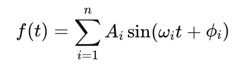
DAM X can embed such oscillations at the mathematical core, using:
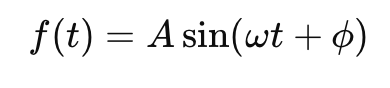
or, for more complex rhythms,
where:
- A: amplitude,
- ω: angular frequency,
- ϕ: phase shift.
These rhythms allow DAM X to represent both regular cycles (like sleep-wake) and irregular, combined cycles (like financial markets with overlapping trends).
Fourier Series and Transformations: Decomposing the Pulse
Not all cycles are simple.
Fourier series allow us to decompose any periodic signal into a sum of sines and cosines:
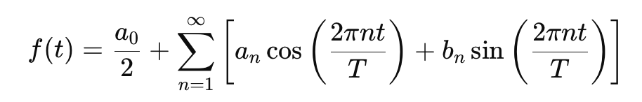
where T is the period.
This gives DAM X the flexibility to discover hidden cycles in data and adapt to new ones as the world changes.
Time-Varying Correlation and Dynamic Dependence
In real systems, the strength and form of relationships change with time.
DAM X allows all copula parameters and dependency structures to evolve dynamically:
Cθ(t)(F1(x1,t),F2(x2,t),…,Fn(xn,t))
where θ(t) encodes how relationships wax and wane with shifting context.
Adaptive Correlation Examples:
Exponentially weighted moving average (EWMA):
Σt=αΣt−1+(1−α)(xtxt⊤)
Regime-Switching Covariance:
Σt=Σ1⋅I(st=1)+Σ2⋅I(st=2)+…+Σm⋅I(st=m)
where stst is a latent regime variable.
Hidden Markov Models: Sensing Regime Changes
Many complex systems jump between distinct modes or regimes:
- Bull vs. bear markets.
- Sleep vs. wake in neural circuits.
- Dry vs. wet seasons in ecology.
Hidden Markov Models (HMMs) provide a probabilistic way to model such switches:
p(st∣st−1)=transition probabilities
p(xt∣st)=emission probabilitiesp
DAM X can use HMMs to adapt its own internal clocks and relationships, sensing when a fundamental shift has occurred.
Spectral Mixture Kernels: Embracing Complexity
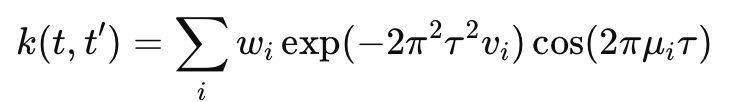
For especially complex, quasi-periodic, or multi-frequency phenomena (e.g., climate cycles, brain rhythms), DAM X can employ spectral mixture kernels:
with τ=∣t−t′∣, weights wi, frequencies μi, and variances vi.
Energy, Entropy, and the Adaptive Clock
DAM X goes further:
It can produce its own sense of time, with internal time density depending on energy and entropy:
- High energy / high entropy: Time speeds up—more adaptation, faster change.
- Low energy / low entropy: Time slows, system stabilizes, perhaps even rests.
This mirrors living systems:
- A predator senses prey, and its brain “speeds up” in anticipation.
- A market senses calm, and volatility contracts—time itself feels slower.
Practical Example: Adaptive Trading Algorithm
Suppose you’re designing an algorithmic trader:
- In periods of high volatility (energy), the system increases its update rate, switching to high-frequency trading strategies.
- In calm markets, it slows down, saves computation, and focuses on long-term trends.
The “clock” of the algorithm is not fixed—it adapts, mirroring the living logic of the market.
Sample Code: Adaptive Time Step Simulation
energy = compute_system_energy(state)
entropy = compute_system_entropy(state)

# Example: Time step adapts to energy/entropy level
dt = base_dt / (1 + energy + entropy)  # Faster when dynamic, slower when calm

for t in np.arange(0, total_time, dt):
    state = update_state(state, dt)
    # ... rest of simulation ...
Conclusion: From Fixed Clocks to Living Rhythms
Time is not a flat backdrop, but a living pulse in DAM X.
- Rhythms, cycles, and regime changes are all part of the adaptive dance.
- The system feels, responds, and even produces its own temporal flow.
To model life, we must let time itself become dynamic—sometimes a gentle river, sometimes a roaring flood.